Create a filtered list according to certain criteria, without degrading the original data
FILTER function
The FILTER function allows you to create another list from a list that is dynamically filtered according to 1 or more criteria.
=FILTER(array, include, [if_empty])
In the arguments of this function,
- array: The area to be restored
- include: Filter Criteria
- if_empty: If the criterion is not found, what should be displayed. (Optional argument)
Using the FILTER function
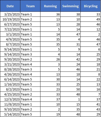
From the list below, let‘s see how to use the Filter function.
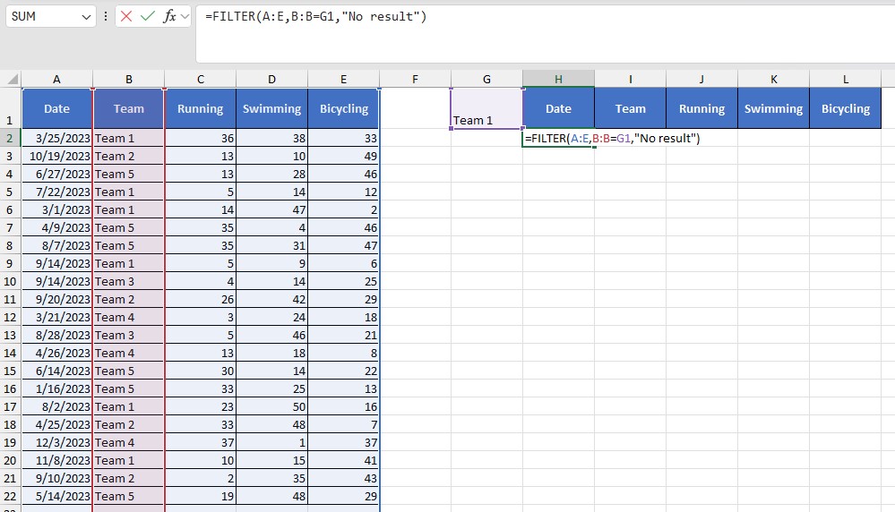
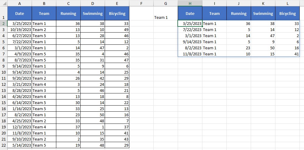
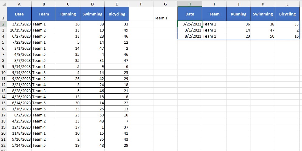
In the example below, we‘re looking to make a list with all the rows in Team 1. To do this, we indicate the filter criterion (G1) in a cell. The title line has been copied.
Note: It is possible to use the Filter function in another tab, or even another file. For the example, we‘ve put it next to the original list.
Then in H2 (beginning of the 2nd list), enter the formula:
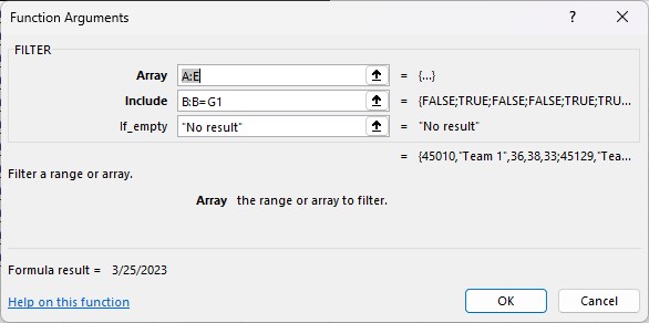
=FILTER(A:E,B:B=G1,”No result”)
We want to render all columns (A:E) but only the rows where team 1 is in the Team column (B:B=G1), but if no row shows Team 1, then we display “No result“.
Simply enter the formula in the 1st cell of the table and it is fully filled.
Warning: The Filter function is a propagating function. The cells next to it must be empty.
If we change the criterion (to cell G1), all the fields in the list are updated.
Filter with multiple criteria
It is possible to apply several criteria to the filter.
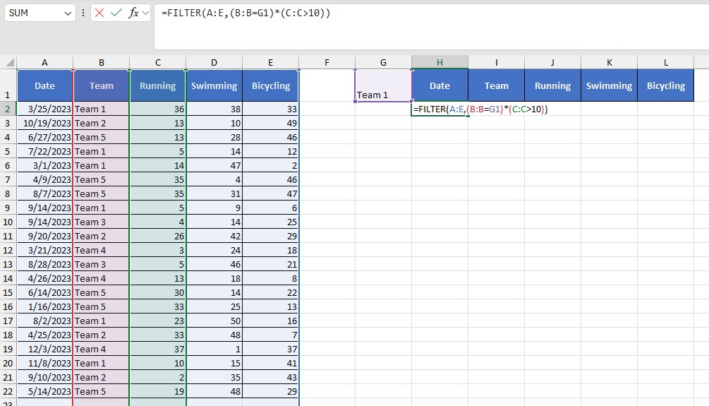
In our example, we want to filter all the rows of team 1 (BB=G1) and whose Race score is greater than 10 (C:C>10). If the criteria are not met, then we chose to display nothing and don’t fill the last argument.
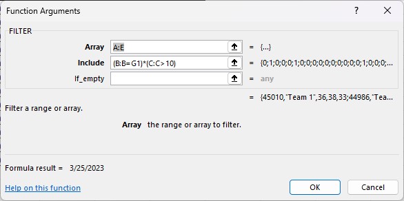
=FILTER(A:E,(B:B=G1)*(C:C>10))
To take into account several criteria, each criterion is put in parentheses and the symbol * allows the different criteria to be linked.
Filter without showing the criterion
With the FILTER function, it is also possible to return a list without the criterion being displayed.
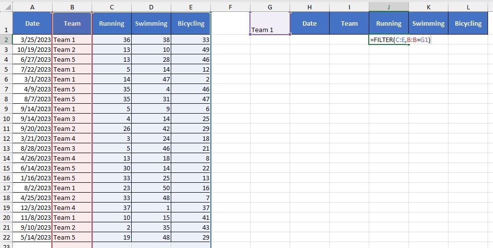
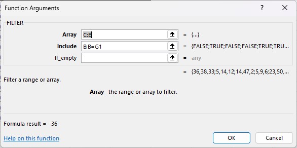
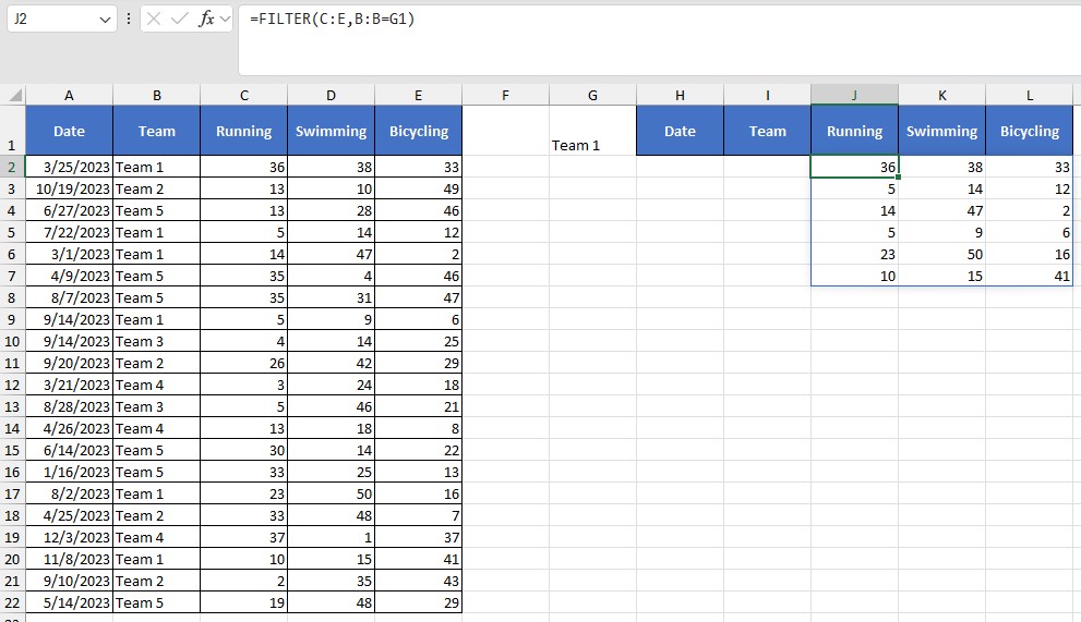
In the example below, we want to show only the Running, Swimming, and Bicycling scores for Team 2, without putting a Date or Team column.
=FILTER(C:E,B:B=G1)
In the formula, we indicate that the table to be rendered is between columns C and E. However, the criterion field is listed in column B.
Note: the restitution table must always be contiguous columns.
The criterion is still in cell G1. But the corresponding column has not been repatriated.
