Pivot tables allow you to group and analyze data, whether you have very large or smaller tables.
From the following table, let‘s look at how to do it.
Creating a PivotTable
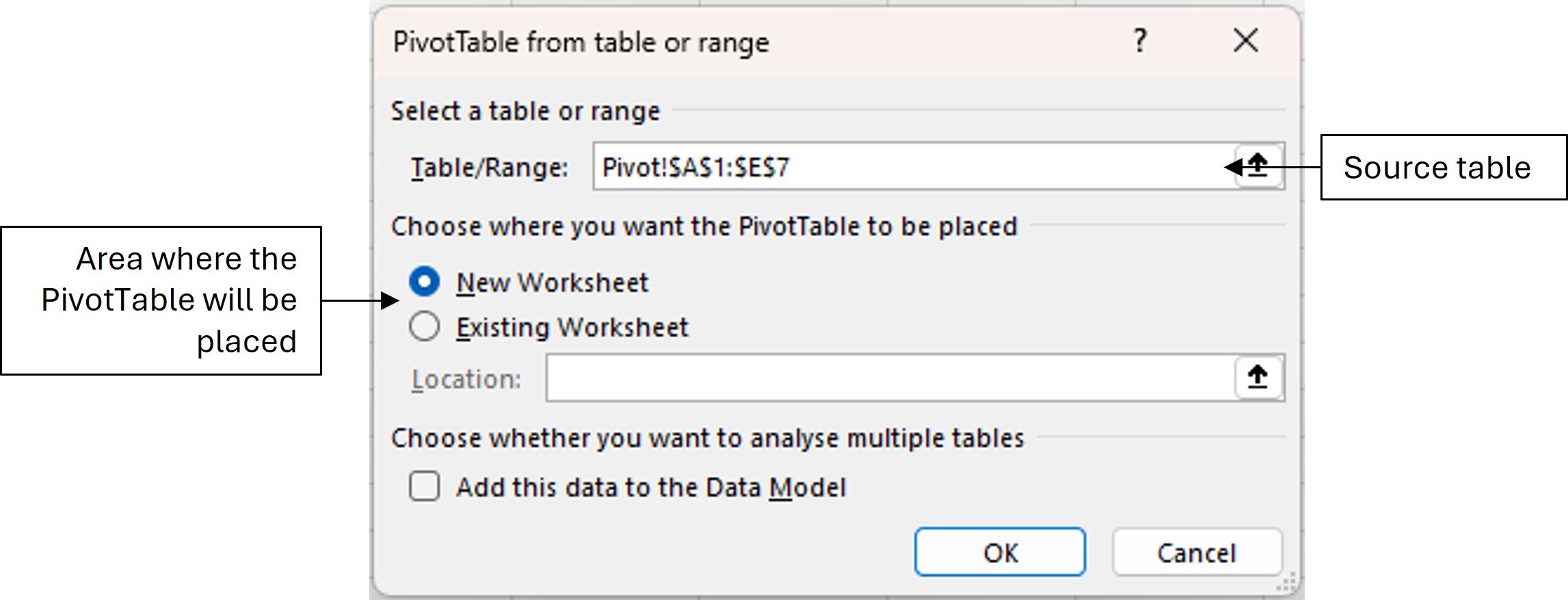
First, select the table. Then on the Insert menu, in the Tables section, click PivotTable.
In the window that opens, the Table/Range box shows the place of the source table. You have to choose where the pivot table will be placed:
- On a new sheet or
- On an existing sheet (specify where exactly)
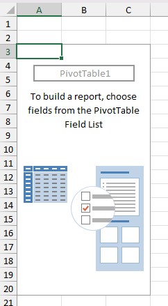
A pivot table is distinguished by two distinct areas: on the left, the layout of the table to be constructed; and on the right, the fields that are utilized for the pivot table.
Construction
In order to build a table, you need to drag the different fields into the boxes.
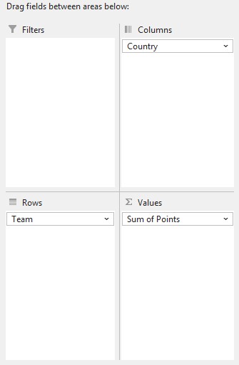
In our example, we want to add up the points per team and per country. So we draggued in:
- The Team field in the Rows area
- The Country field in the Columns area
- The Points field in the Values area (by default a sum is made but it is possible to change the calculation)
Depending on the message you want, it is possible to set up the pivot table differently.
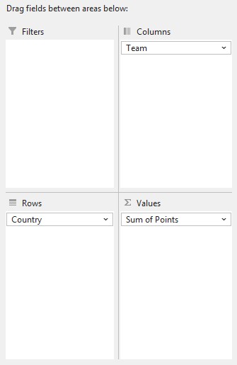
Indeed, in this new example, we want to add up the points per country and per team.
So we drag in:
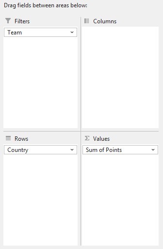
- The Country field in the Rows area
- The Team field in the Columns area
- The Points field in the Values area (by default a sum is made but it is possible to change the calculation)
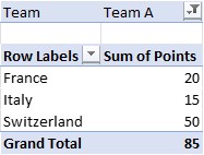
The Filters area allows you to view data for one (or more) category(ies). To do this, drag the field you want in it.
Refresh the PivotTable
If the source data is changed, the PivotTable will not be changed. To make the table reflect the changes, click in the PivotTable and then click Refresh.
If you don‘t know how to cross-reference your data, you can ask Excel for help: Excel: Recommended PivotTables


