Excel’s SORT and SORTBY functions: Generate a list sorted by specific criteria without altering the original data.
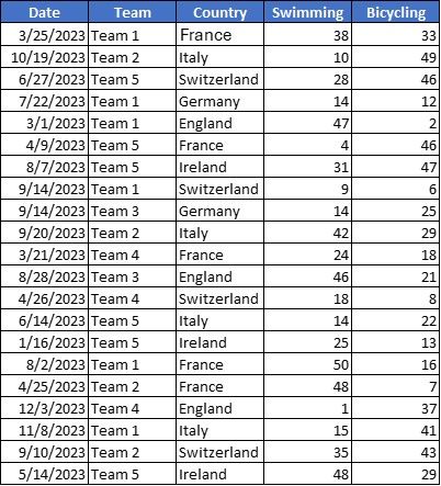
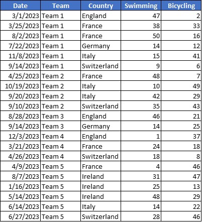
The use cases of these 2 functions will be based on the following table.
Note: These functions are functions that propagate. Just enter them once to fill an entire column or table. Make sure you have enough space available.
SORT Function
The SORT function allows you to create another dynamically sorted list from a list.
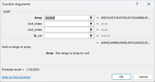
=SORT(array, [sort_index], [sort_order], [by_col])
In the arguments of this function,
- array: The area to be rendered (1 column or a table)
- sort_index: Which column should be sorted from (Optional argument)
- sort_order: Sort in ascending order (1) or descending (–1) (Optional argument)
- by_col: Set FALSE by default (sorting by lines) (Optional argument and not necessary)
Using the SORT Function
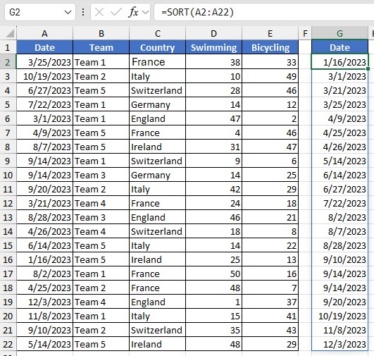
In the list to be returned, the column title must already be entered. All selected data is sorted.
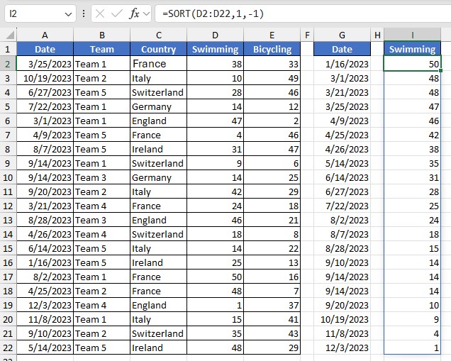
Sort a column in ascending (or chronological) order
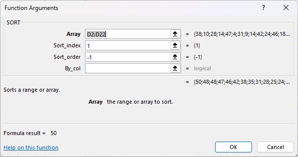
Sort a column in descending order
Sorting in a table
It can also be interesting to render an entire table with a sort, rather than a single column.
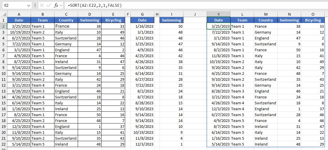
First, we duplicate the column headers. Then we go to the 1st cell (under the header in the leftmost column) and type:
=SORT(A2:E22;2;1;FALSE)
We indicate that we take the whole table (A2:E22), that the sorting will be done on the 2nd column (Team) in ascending order (1) and that it will be done by row (False).
SORTBY Function
To render an entire array, the SORTBY function is simpler than the SORT function.
The SORTBY function allows you to create another table from a table, but whose columns are dynamically filtered according to 1 or more criteria.
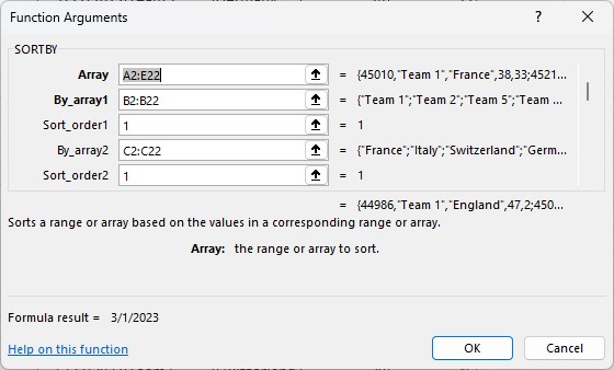
=SORTBY(array, by_array1, [sort_order], [by_array2, sort_order2], [by_array3, sort_order3], …)
In the arguments of this function,
- array: The area to be restored (reference table)
- by_array1: 1st column to sort
- sort_order: Sort in ascending (1) or descending (–1) order (Optional argument)
- by_array2: 2nd column to sort (Optional argument)
- sort_order2: Sort in ascending (1) or descending (–1) order (Optional argument)
- by_array3: 3rd column to sort (Optional argument)
- sort_order3: Sort in ascending (1) or descending (–1) order (Optional argument)
It is possible to go up to 127 sorts!
Using the SORTBY Function
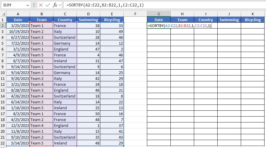
In the example below, we want to render the same table as the reference one, but with all the teams in ascending order and the countries as well.
So we place ourselves in cell G2 (just below the title). Then we enter:
=SORTBY(A2:E22;B2:B22;1;C2:C22;1)
The data is rendered in a raw way. After formatting the titles and then applying a date format to the 1st column, here is the result.
